9/5/2019

Building an orbital mechanics simulator

As a part of my bachelor's thesis I decided I wanted to simulate the orbital dynamics of a 3U cubesat for the evaluation of different thrusting strategies using low thrust maneuvers.

Part 1: Core

Im really not an expert in computational physics so I simply started using python's integrate.solve_ivp integrator. This function requires a differential equation to integrate and in this case I started using Cowell's formulation, which can be expressed as follows:

\frac{d}{dt}\begin{bmatrix}\mathbf{r} \\ \mathbf{v}\end{bmatrix} = \begin{bmatrix}\mathbf{v} \\ \mathbf{a}\end{bmatrix} = \begin{bmatrix}\mathbf{v} \\ -\mu\frac{\mathbf{r}}{r^3}+\mathbf{p}\end{bmatrix}

where $\mathbf{r}$ is the position vector, $\mathbf{v}$ is the velocity vector, $\mu$ is the standard gravitational parameter of the center body (the Earth in this case) and $\mathbf{p}$ is the acceleration vector due to perturbations (more on that later, we'll assume it as zero for now).

This expression translates to the function as below. Because the integrating function must accept only one variable for integration, I had to pass all the variables in a single state vector in the input and output, which is kinda ugly but works ok.

def cowell(t, stateVector):
    r = stateVector[0:3]
    v = stateVector[3:6]
    p = 0

    #Differential Equations
    drdt = v
    dvdt = mu_E*(r/(np.linalg.norm(r)**3))+p

    return np.append(drdt,dvdt)

Having defined our integration function, we can then use it in our propagation function. This function I've called it propagate as that's normally the term used in the simulators. This function takes in the amount of time we want to propagate, and the timestep we want the resulting time series to be in.

def propagate(y0, time,timestep):
    t = np.linspace(0,time,time/timestep)
    sol = integrate.solve_ivp(cowell, (t[0],t[-1]), y0, t_eval=t, method='LSODA')
    return sol

And that's it. That's all we need to do a very barebones orbital dynamics simulator, you can now do:

# define initial position and velocity (you'll have to trust me for now with this parameters)
# they represent values in m and m/s respectively
r = [12861487, 7953413, 263915]
v = [-824, 3650, 2063]
y0 = np.append(r,v)
# propagate for an interval of 3.4 hours with a 1 minute resolution:
sol = propagate(y0, 60*60*3.4, 60)

# Plotting, I've used ipyvolume for this.
fig = ipv.figure(width=800,height=500)
ipv.plot(sol.y[0,:]/1e3,sol.y[2,:]/1e3,sol.y[1,:]/1e3)
ipv.pylab.style.box_off()
ipv.pylab.xyzlim(10e3)
display(fig)

to obtain a nicely looking orbit like this:

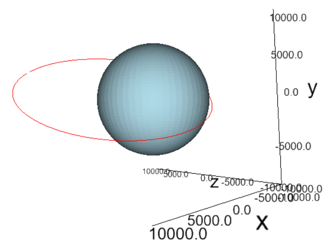
A simple orbit — Neat! (Note: I've added a sphere as an extra to represent the Earth)

Part 1.5: Cleaning Up

Before continuing I wanted to better organize the code to make it smarter and more maintainable. So I decided to split it into 3 main files:

constants.py: to store all the constants used in astronomy, so then I could just call constants._<constant_name>_
coordinates.py: to store all the functions that transform between the many coordinates systems used in astronomy.
maneuvers.py: I decided I would treat a whole maneuver as a class which stores its state internally, and therefore I would place it in its own file.
models.py: to store all the functions which represent physical models of spacecraft components, physical phenomena, etc.

The first one was easy:

# constants.py

import numpy as np

# Universal Gravity
G = 6.67e-11
# Astronomical unit (m):
AU = 149597870691

#EARTH
# Earth Mass
Me = 5.97e24
#Earth Radius
Re = 6378e3
#Earth Angular Speed
wE = np.array([0,0,7.2921159e-5])
#Gravity Constants
mu_E = G*Me
#g0 constant (m/s)
g0 = 9.806

For the second one I wanted to be able to transform Keplerian Elements to Cartesian Elements. This is because, when speaking about orbiting bodies, it's a lot easier to visualize everything in terms of keplerian elements than cartesian ones.

If you wish to learn about keplerian elements, you can checkout the wikipedia page by clicking the image below

So I made the transformation function according to this cheatsheet:

# coordinates.py

import numpy as np

def kep2cart(coe):
    """ Keplerian to Cartesian """
    a = coe[0]
    e = coe[1]
    i = coe[2]
    omega = coe[3]
    Omega = coe[4]
    nu = coe[5]

    E = 2*np.arctan2(np.tan(nu/2),np.sqrt((1+e)/(1-e)))

    mu = constants.mu_E
    rc = a*(1-e*np.cos(E))
    o = rc*np.array([np.cos(nu),np.sin(nu)])
    odot = (mu*a)**0.5/rc*np.array([-np.sin(E), (1-e**2)**0.5*np.cos(E)])
    rotationMatrix =  np.array(
            [[np.cos(omega)*np.cos(Omega)-np.sin(omega)*np.cos(i)*np.sin(Omega), -(np.sin(omega)*np.cos(Omega)+np.cos(omega)*np.cos(i)*np.sin(Omega))],
             [np.cos(omega)*np.sin(Omega)+np.sin(omega)*np.cos(i)*np.cos(Omega),   np.cos(omega)*np.cos(i)*np.cos(Omega)-np.sin(omega)*np.sin(Omega)],
             [np.sin(omega)*np.sin(i), np.cos(omega)*np.sin(i)]])
    r = np.matmul(rotationMatrix,o)
    v = np.matmul(rotationMatrix,odot)

    return r,v

For the third one, I implemented a Maneuvers class using the same things mentioned in Part 1:

# maneuvers.py

import numpy as np
import constants, coordinates
import ipyvolume as ipv
from scipy import integrate

class Maneuvers:
    def __init__(self, coe, initTime):
      self.coe = coe
      self.r, self.v = coordinates.kep2cart(coe)
      self.initTime = initTime

    def propagate(self, time,timestep):
        t = np.linspace(self.initTime,time,time/timestep)
        y0 = np.append(self.r,self.v)
        sol = integrate.solve_ivp(self.cowell, (t[0],t[-1]), y0, t_eval=t, method='LSODA')
        self.rSol = sol.y[0:3,:]

    def plot3D(self):
        fig = ipv.figure(width=800,height=500)
        ipv.plot(self.rSol[0,:]/1e3,
                 self.rSol[2,:]/1e3,
                 self.rSol[1,:]/1e3)
        ipv.pylab.style.box_off()
        ipv.pylab.xyzlim(10e3)

    def cowell(self, t, stateVector):
        r = stateVector[0:3]
        v = stateVector[3:6]
        p = 0

        #Differential Equations
        drdt = v
        dvdt = constants.mu_E*(r/(np.linalg.norm(r)**3))+p

        return np.append(drdt,dvdt)

After that I could simply do:

# main.py

import Maneuvers from maneuvers

 #----- INITIAL CONDITIONS -----
# Explicit conditions
rp = constants.Re+230e3
ra = constants.Re+1000e3
Omega = 30*np.pi/180
i = 2*np.pi/180#65.1*np.pi/180
omega = 30*np.pi/180
M = 332*np.pi/180
#-------------------
# Derived conditions
e = (ra-rp)/(ra+rp)
a = (ra+rp)/2
#--------------------
coe = [a,e,i,omega,Omega,M]
initTime = 0
# Create maneuver
maneuver = Maneuvers(coe, initTime)
# Propagate for 3.4 hours
maneuver.propagate(60*60*3.4,60)
# Plot
maneuver.plot3D()

After all of this, we should be able to get the same plot as before but with a much cleaner interface

Part 2: Putting in some meat

(This part is not that fun, and you can skip it if you like)

What we have so far is cool, but it still is very basic. Space is a mess of forces acting in every direction, of which some are more relevant than others.

In that case I'll continue by adding some perturbations to the simulation.

Orbiting bodies in space don't actually describe a perfect ellipse all the time. In fact they're constantly being perturbed out of equilibrium by the other massive object around it.

There're 5 major perturbations in LEO (Lower Earth Orbit):

Atmospheric Drag: caused by the atmospheric density from 600 km of altitude and below. The atmospheric particles in the atmosphere crash against the orbiting body at a very high speed, slowing it down until it crashes to the Earth. In a similar fashion than how a parachute slows you down.

The acceleration due to this force is expressed as:

\mathbf{p} = -\frac{1}{2}\rho v_{rel}\bigg(\frac{C_DA}{m}\bigg)\mathbf{v}_{rel}

where $\rho$ is the atmospheric density, $v_{rel}$ is the relative speed between the body and the air, $C_D$ is the drag coefficient of the body, and $\big(\frac{C_DA}{m}\big)$ is the inverse of the ballistic coefficient of the body.

The trickiest part to get right is the atmospheric density, which is dependant on many factor and many models have been proposed. However, I decided to just use the USSA76 model, one of the oldest, most basic and most used models. There are many more elaborate atmospheric models out there, but for the time being we'll only use this one.

This model has been tabulated and therefore coded it using the tabulated values, and using an exponential interpolation to obtain the values in between:

# models.py
def USSA76(z):
    """
    US Standard Atmosphere 1976. Exponential interpolation.
    Ref: https://ntrs.nasa.gov/archive/nasa/casi.ntrs.nasa.gov/19770009539.pdf
         https://www.mathworks.com/matlabcentral/mlc-downloads/downloads/submissions/52703/versions/1/previews/atmosphere.m/index.html
         Orbital Mechanics For Engineers, Curtis 2013
    """
    z = z/1e3

    i=0
    h = [ 0, 25, 30, 40, 50, 60, 70, 80, 90, 100, 110, 120, 130, 140, 150, 180, 200, 250, 300, 350, 400, 450, 500, 600, 700, 800, 900, 1000];
    rho = [1.225, 4.008e-2, 1.841e-2, 3.996e-3, 1.027e-3, 3.097e-4, 8.283e-5, 1.846e-5, 3.416e-6, 5.606e-7, 9.708e-8, 2.222e-8, 8.152e-9, 3.831e-9, 2.076e-9, 5.194e-10, 2.541e-10, 6.073e-11, 1.916e-11, 7.014e-12, 2.803e-12, 1.184e-12, 5.215e-13, 1.137e-13, 3.070e-14, 1.136e-14, 5.759e-15, 3.561e-15];
    H = [ 7.310, 6.427, 6.546, 7.360, 8.342, 7.583, 6.661, 5.927, 5.533, 5.703, 6.782, 9.973, 13.243, 16.322, 21.652, 27.974, 34.934, 43.342, 49.755, 54.513, 58.019, 60.980, 65.654, 76.377, 100.587, 147.203, 208.020];
    for j in range(0,27):
        if z >= h[j] and z < h[j+1]:
            i = j
    if z == 1000:
        i = 27
    density = rho[i]*np.exp(-(z-h[i])/H[i]);
    return density

The code expression for the drag is then:

# Calculate altitude to obtain atm density
z = np.linalg.norm(r) - constants.Re
# Calculate relative velocity to atmosphere using Earth's angular velocity
vrel = v - np.cross(constants.wE,r)
# Get atm density using altitude
rho = models.USSA76(z)
# Calculate Drag
Fd = -0.5*rho*np.linalg.norm(vrel)*vrel*(1/BC)

Sun and Moon gravity: caused (you guessed it) by the Sun an Moon's gravity. In the case of the Moon, the acceleration caused by this force is expressed as:
$\mathbf{p} = \mu_m\bigg(\frac{\mathbf{r}_{m/s}}{r_{m/s}^3}-\frac{\mathbf{r}_m}{r_m^3}\bigg)$
where $\mu_m$ is the Moon's standard gravitational parameter, $\mathbf{r}_{m/s}$ is the position of the moon relative to the satellite, and $\mathbf{r}_m$ is the position of the Moon relative to Earth.

In order to calculate the position of the Moon with respect to the Earth, I used this algorithm, which I adapted to python here.
```
r_m = models.lunarPositionAlmanac2013(self.history.datetime[0]+timedelta(seconds=t))
r_ms = r_m-r
pMoon = constants.mu_M*(r_ms/np.linalg.norm(r_ms)**3-r_m/np.linalg.norm(r_m)**3)
```
In case of the perturbation caused by the Sun, the expression is the same but considering its position and gravitational parameter instead of the Moon's.
Solar Radiation Pressure: believe it or not, the light delivered by the Sun does impose a force in the bodies it illuminates. This is because even though photons don't have any mass, they transmit momentum.

Because this force is so minuscule, we don't percieve it on Earth, but it does have a greater effect in outer space, especially if you consider satellites are decades orbiting the Earth.

The expression for the acceleration generated by Solar Radiation Pressure can be modeled as:
$\mathbf{p} = -\nu\frac{S}{c}\frac{C_RA_S}{m}\mathbf{\hat{u}}$
where $\nu$ is the shadow function, which has a value of 0 if the satellite is in the shadow of the Earth, and 1 otherwise. $C_R$ is the Radiation Pressure Coefficient, which is a value between 1 and 2 depending on the body's surface capacity to absorb or reflect photons. $A_S$ is the exposed area, $m$ is the body's mass, $S$ the Radiation Intensity at 1AU of the Sun ( $1367 W/m^2$ ) and $c$ is the speed of light constant.
```
#u-hat vector pointing from Sun to Earth and Sun position vector
uhat, rS = models.solarPosition(self.history.datetime[0]+timedelta(seconds=t))

#Solar Radiation Pressure
PSR = 4.56e-6
#Absorbing Area
As = self.spacecraft.area

#Shadow function
rSNorm = np.linalg.norm(rS)
rNorm = np.linalg.norm(r)
theta = np.arccos(np.dot(rS,r)/(rSNorm*rNorm))
theta1 = np.arccos(constants.Re/rNorm)
theta2 = np.arccos(constants.Re/rSNorm)
if(theta1+theta2 > theta):
  nu = 1
else:
  nu = 0

#Radiation Pressure Coefficient (lies between 1 and 2)
Cr = self.spacecraft.Cr
#Spacecraft mass
mass = self.spacecraft.dryMass+propMass
#Radiation Pressure acceleration
FR = -nu*PSR*Cr*As/mass*uhat
```
Earth Harmonic J2: because the earth is not round but a bit squashed in the poles, the gravitational field does not distribute uniformly in all directions. These are called gravitational harmonics. The most relevant harmonic is J2 harmonic.
$\mathbf{p} = \frac{3}{2}\frac{J_2\mu R^2}{r^4}\bigg[\frac{x}{r}\bigg(5\frac{z^2}{r^2}-1\bigg)\mathbf{\hat{i}}+\frac{y}{r}\bigg(5\frac{z^2}{r^2}-1\bigg)\mathbf{\hat{j}}+\frac{z}{r}\bigg(5\frac{z^2}{r^2}-3\bigg)\mathbf{\hat{k}}\bigg]$
```
J2 = 0.00108263

zz = r[2]

rNorm = np.linalg.norm(r)
bigTerm = np.array([1/rNorm*(5*zz**2/rNorm**2-1),
                    1/rNorm*(5*zz**2/rNorm**2-1),
                    1/rNorm*(5*zz**2/rNorm**2-3)])

#J2 Gravity Gradient
FJ2 = (3/2)*J2*constants.mu_E*constants.Re**2/rNorm**4*bigTerm*r
```

Part 3: Changing the propagation method

By the time I reached this point, I started noticing something a strange behaviour in the simulation. So I tested what would happen if I did propagated the model for a long time without any perturbations.

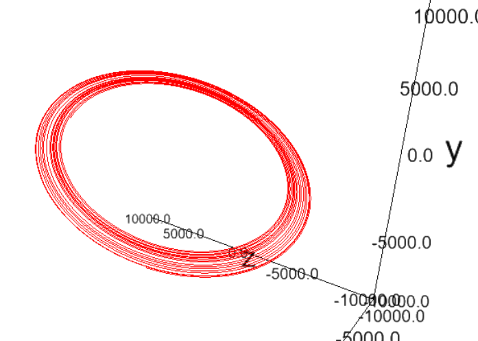
As suspected the orbit starts to slowly move away from its original parameters. I attributed this to the numerical error introduced by Cowells method.

I needed something more stable, so I thought on changing the formulation to Gauss Formulation instead of Cowells.

After some hours reading papers on the matter, I found out there's a way to represent the position of an object in space that is alternative to the Keplerian/Classical Orbital Elements.

This type of elements are called Equinoctial Elements and they were invented to solve some of the problems Keplerian elements presented. They're defined as follows:

\begin{align} p & = a(1-e^2)\\ f & = e\cos(\omega+\Omega)\\ g & = e\sin(\omega+\Omega)\\ h & = \tan(\frac{i}{2})\cos(\omega)\\ k & = \tan(\frac{i}{2})\sin(\Omega)\\ L & = \omega+\Omega+\nu \end{align}

I also figured out that you can use this elements to describe the motion of the body: $\dot{x} = A(x)\Delta+b$ where:

x = \begin{bmatrix}p & f & g & h & k & L\end{bmatrix}^T A = \begin{bmatrix} 0 & \frac{2p}{q}\sqrt{\frac{p}{\mu}} & 0\\ \sqrt{\frac{p}{\mu}}\sin L & \sqrt{\frac{p}{\mu}}\frac{1}{q}[(q+1)\cos L +f] & -\sqrt{\frac{p}{\mu}}\frac{g}{q}(h\sin L - k\cos L) \\ -\sqrt{\frac{p}{\mu}}\cos L & \sqrt{\frac{p}{\mu}}\frac{1}{q}[(q+1)\sin L +g] & \sqrt{\frac{p}{\mu}}\frac{f}{q}(h\sin L - k\cos L) \\ 0 & 0 & \sqrt{\frac{p}{\mu}}\frac{s^2\cos L}{2q} \\ 0 & 0 & \sqrt{\frac{p}{\mu}}\frac{s^2\sin L}{2q} \\ 0 & 0 & \sqrt{\frac{p}{\mu}}\frac{1}{q}(h\sin L - k\cos L) \\ \end{bmatrix} b = \begin{bmatrix} 0 & 0 & 0 & 0 & 0 & \sqrt{\mu p}\big(\frac{q}{p}\big)^2 \end{bmatrix}^T

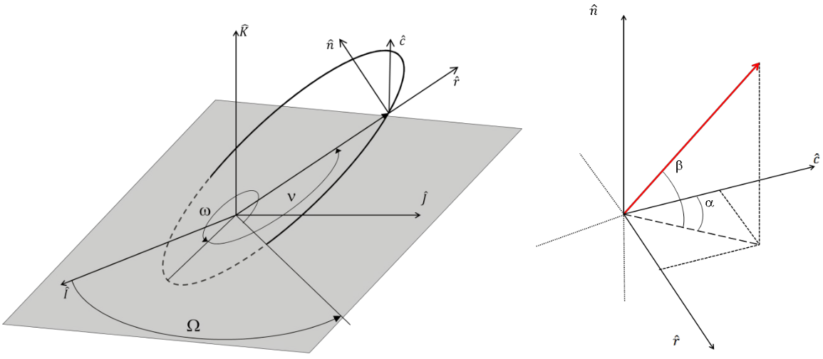
and $\Delta$ , the perturbations in the RSW frame of reference (radial-traverse-normal) of the spacecraft. This frame of reference is also sometimes called RCN, and looks something like this:

Because all the previous perturbations were described in the ECI (Earth-Centered-Inertial) frame of reference, I had to transform all of them to the new frame of reference doing a simple dot product:

#RSW frame definition from r and v
rhat = r/np.linalg.norm(r)
w = np.cross(rhat,v)
what = w/np.linalg.norm(w)
shat = np.cross(what,rhat)
rsw = [rhat, shat, what]
#Transform perturbations to RSW Frame
Delta = np.dot(rsw,pert)

A = np.array([[0, 2*p/q*np.sqrt(p/constants.mu_E),0],
              [np.sqrt(p/constants.mu_E)*np.sin(L), np.sqrt(p/constants.mu_E)*1/q*((q+1)*np.cos(L)+f), -np.sqrt(p/constants.mu_E)*g/q*(h*np.sin(L)-k*np.cos(L))],
              [-np.sqrt(p/constants.mu_E)*np.cos(L), np.sqrt(p/constants.mu_E)*(1/q)*((q+1)*np.sin(L)+g), np.sqrt(p/constants.mu_E)*(f/q)*(h*np.sin(L)-k*np.cos(L))],
              [0, 0, np.sqrt(p/constants.mu_E)*s**2*np.cos(L)/(2*q)],
              [0, 0, np.sqrt(p/constants.mu_E)*s**2*np.sin(L)/(2*q)],
              [0, 0, np.sqrt(p/constants.mu_E)*(1/q)*(h*np.sin(L)-k*np.cos(L))]])
b = np.array([0, 0, 0, 0, 0, np.sqrt(constants.mu_E*p)*(q/p)**2])

dotx = np.matmul(A,Delta) + b
return dotx

This ultimately yielded a lot better results, and it also calculated everything much faster 😁.

Part 4: Adding in Thrust

If you think about it, thrust is nothing more than another perturbation, and it just happens to be easier to define it in the RSW frame of reference. So adding it in to the mix is as simple as doing:

DeltaP = [0, thrust/mass, 0]

This will add thrust in the forward direction (the S component in RSW). But of course, we would also like to be able to steer the thrust in order to be able to thrust in all kind of directions.

So I added two directing angles, alpha and beta, which are actually the same you see in the RSW frame definition figure above.

These can be used along with a vector in order to rotate the thrust vector:

\begin{bmatrix} \cos(\beta)\sin(\alpha) & \cos(\beta)\cos(\alpha) & \sin(\beta) \end{bmatrix}^T

The modified expression then becomes:

#Thrust vectoring
RCNThrustAngle = np.array([np.cos(beta)*np.sin(alpha),
                           np.cos(beta)*np.cos(alpha),
                           np.sin(beta)])
DeltaP = thrust/mass*RCNThrustAngle

Part 5: Doing some fancier stuff with thrust

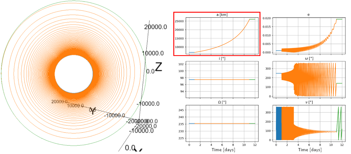
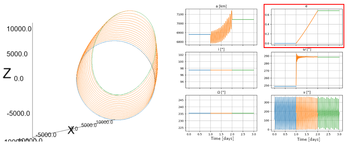
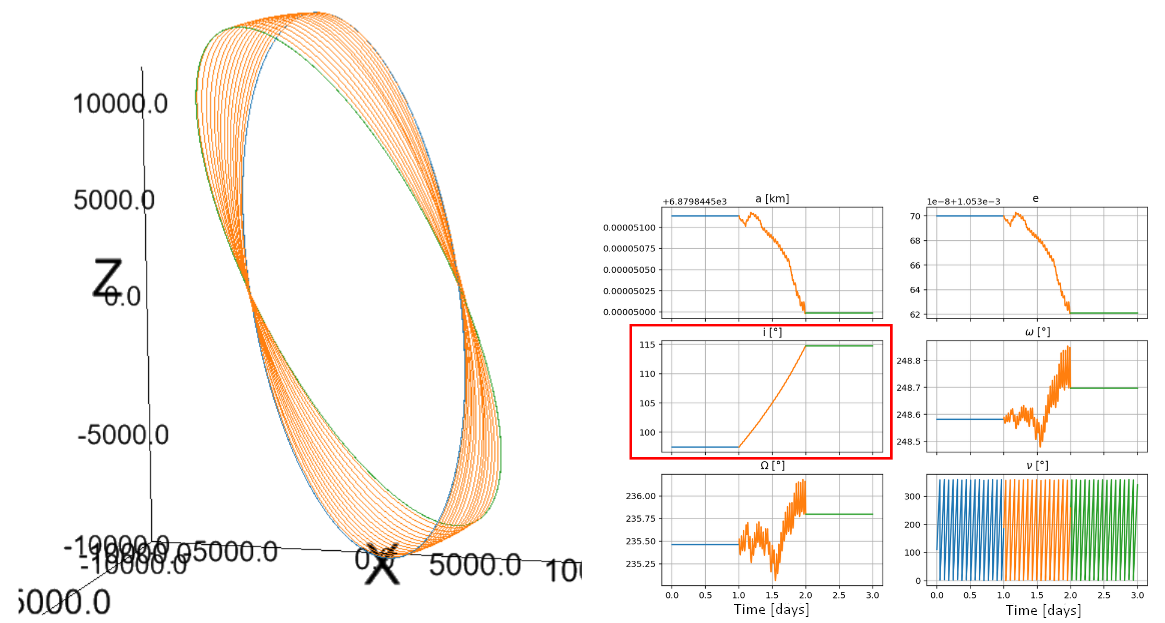
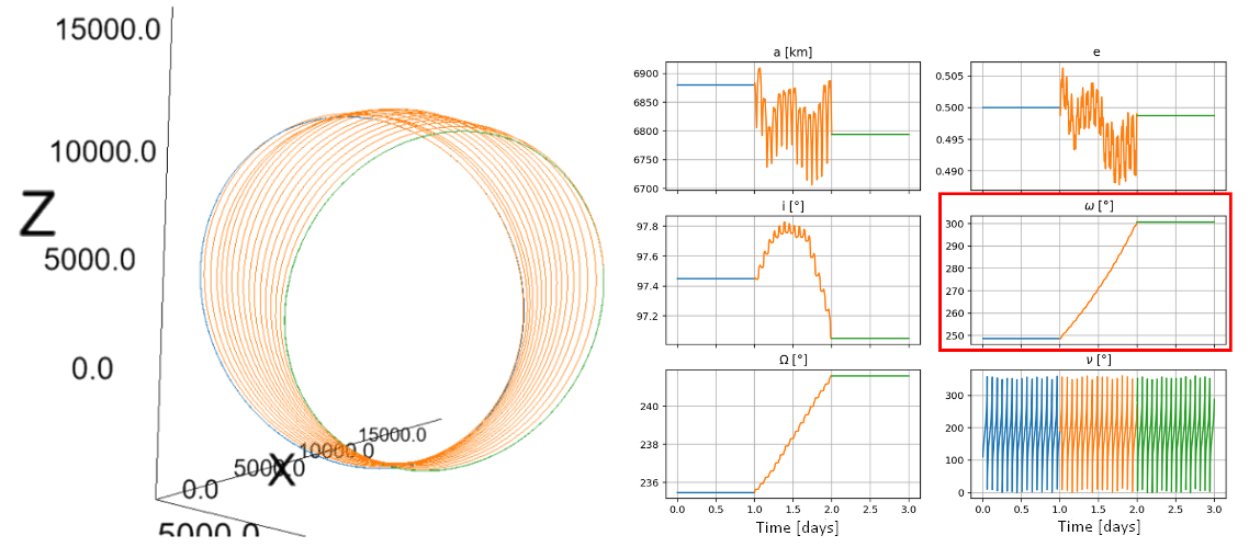
While reading some more papers, I discovered that there's actually some rather old studies on the optimal thrust to modify each of the keplerian elements. These profiles are expressed in the rsw frame of reference, which is something like this:

\begin{array}{|l|c|c|} \hline & \alpha & \beta \\ \hline \textbf{Semi-major axis($a$)} & tan^{-1}\bigg(\frac{e\sin(\nu)}{1+e\cos(\nu)}\bigg) & 0 \\ \hline \textbf{Eccentricity ($e$)} & tan^{-1}\bigg(\frac{\sin(\nu)}{\cos(\nu)+\cos(E)}\bigg) & 0\\ \hline \textbf{Inclination ($i$)} & 0 & \mathrm{sgn}(\cos(\omega+\nu))\cdot\frac{\pi}{2} \\ \hline \textbf{RAAN ($\Omega$)} & 0 & \mathrm{sgn}(\sin(\omega+\nu))\cdot\frac{\pi}{2} \\ \hline \textbf{Argument of perigee ($\omega$)} & \tan^{-1}\bigg(\frac{1+e\cos(\nu)}{2+e\cos(\nu)}\cot({\nu})\bigg) & \tan^{-1}\bigg(\frac{e\cot(i)\sin(\omega+\nu)}{\sin(\alpha-\nu)(1+e\cos(\nu)-\cos(\alpha)\sin(\nu)}\bigg) \\ \hline \end{array}

They seem to be rather complicated, but if we actually plot them we can observe them better. In the images below, for each orbital element, the profiles for the $\alpha$ and $\beta$ angles with respect to the true anomaly $\theta$ . In the right is the visualization in a 2D or 3D space, the black arrows would be the direction of movement (velocity vectors) and the red arrows the direction of thrust (thrust vectors).

Part 6: Pseudo-targeting an orbit

Using the previous profiles to modify a single orbital element, we can combine them to pseudo-target an orbit. This works by calculating the difference/error of each orbital element and weighing more the profile which modifies that particular orbital element.

This way, the orbital element which is lagging to achieve it's target will get corrected quicker because it has greater weight. This can be represented as follows:

\mathbf{T} = \sum_{\mathrm{COE}}\frac{\mathrm{COE}_1-\mathrm{COE}}{\mathrm{COE}_1-\mathrm{COE}_0}\mathbf{T}_{COE}

where $\mathrm{COE}$ , $\mathrm{COE}_1$ and $\mathrm{COE}_0$ represent, respectively, the specific osculating, target and initial orbital element. And $\mathbf{T}$ is the resulting thrust vector of the weighing of every vector. Which in matrix form can be represented as:

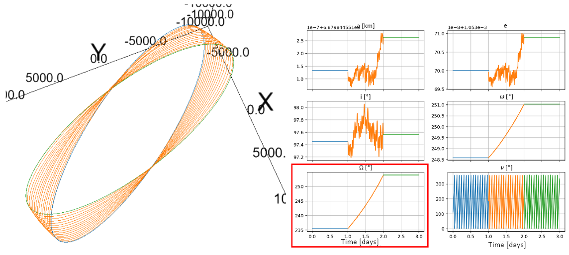
\begin{align} w_{\mathrm{COE}} & = \frac{\mathrm{COE}_1-\mathrm{COE}}{\mathrm{COE}_1-\mathrm{COE}_0}\\ \mathbf{T} & = \left[ \begin{array}{c|c|c|c|c} & & & & \\ \mathbf{T}_a & \mathbf{T}_e & \mathbf{T}_i & \mathbf{T}_\omega & \mathbf{T}_\Omega\\ & & & & \\ \end{array}\right] \begin{bmatrix} w_a\\w_e\\w_i\\w_\omega\\w_\Omega \end{bmatrix} \end{align}

So if we define, for example, an initial orbit with $a_0 = 6879.84$ km, $e_0 = 0.001054$ , $i_0 = 1^\circ$ , and a target orbit with $a_f=13000$ km, $e_f = 0.5$ and $i_f = 45^\circ$ . We get the following result:

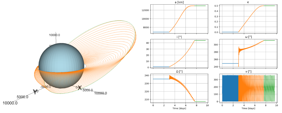
Okay, I think this is getting too long, so I guess I'll just end it here. Hope you've liked it.

Part 7: Wrapping it all up

In case you got lost, you can get the full picture at my github repo. It actually has a lot more things added, but maybe you can understand it with what I've explained here.

Cheers!